Denoising Functions in Matlab With FFT

Reducing the noise of a signal in Matlab using fast fourier transform.

You can download the Matlab file: denoise.m

The function generating the signal in this post will be:

% number of signal measurements
n = 1000;
% measuring from 0 to 2 pi
length = 2*pi;
% difference between two measurements
h = length/n;
% steps
t = (0:h:length-h);
% Signal
S = sin(2*t)+cos(7*t)-cos(t);

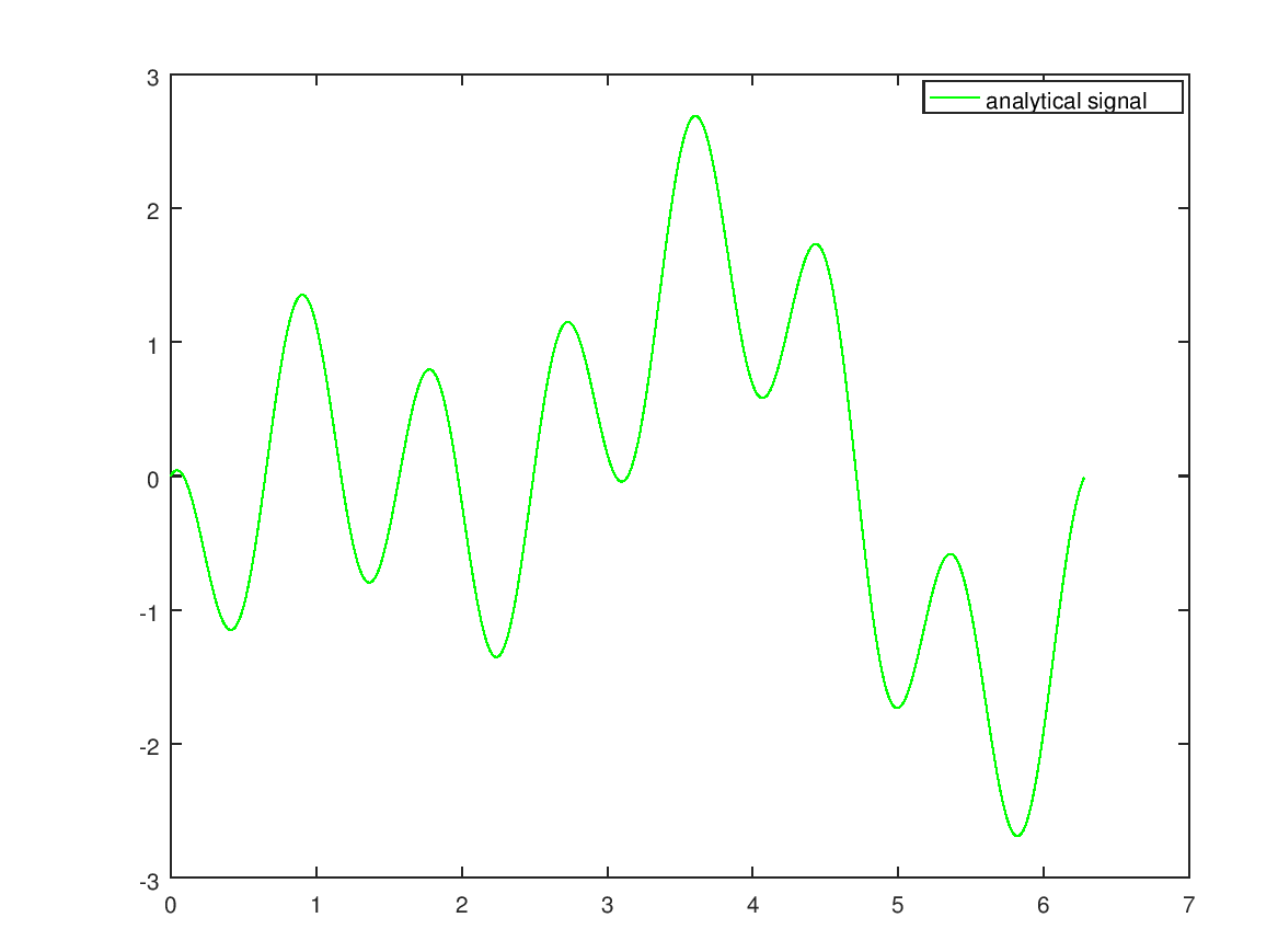
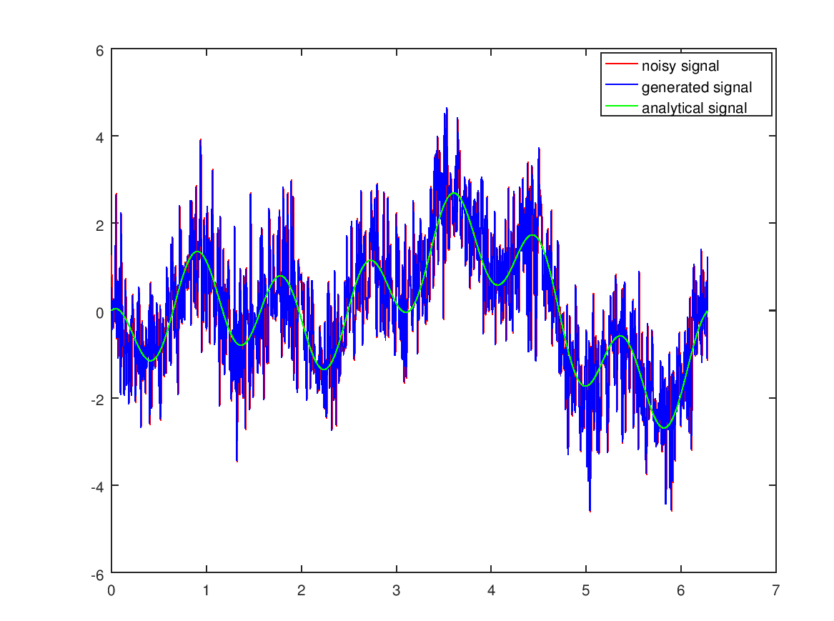
Plot of the signal from 0 to 2*pi.

% random noise
RN = randn(n,1);
% adding the random noise to the signal
NS = transpose(RN) + S;

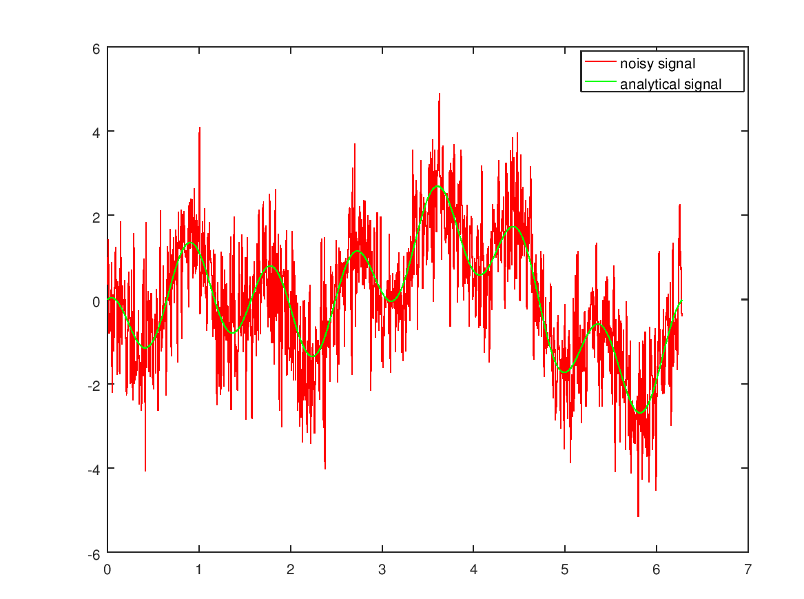
The signal with added noise.

Next we get the complex fourier coefficients using fft. Those get split up into:

Using ak and bk from 1 to s we can put them into the sin cos form of the fourier series.

% getting the complex fourier coefficients using fft
ck = fft(NS);

% dividing the complex fourier coefficients by n 
ck = ck/n;

% setting any complex fourier coefficients smaller than 0.9 times the
% max to zero to remove the noise
m = max(ck);
for i = 1:n
  if ck(i) < 0.9*m
    ck(i) = 0;
  end
end


% getting the fourier coefficients ak and bk
s = floor(n/2)+1;
for i = 1:s
  ak(i) = 2 * real(ck(i));
  bk(i) = -2 * imag(ck(i));
end

% applying the fourier series in sin cos form
for i = 1:n
  y(i) = ak(1)/2;
  for j = 2:s
    y(i) += ak(j) * cos((j-1)*i*h) + bk(j) * sin((j-1)*i*h);
  end
end

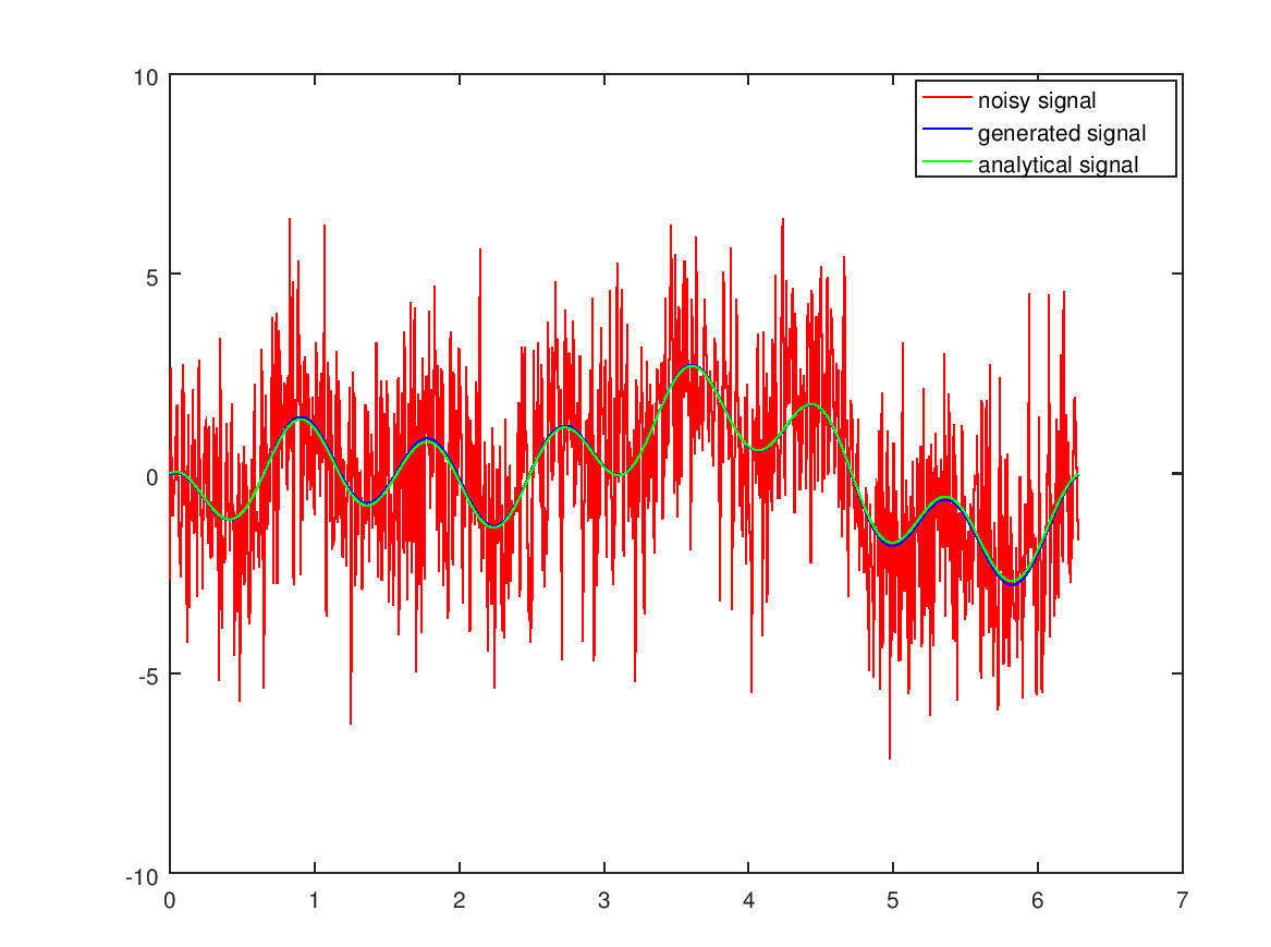
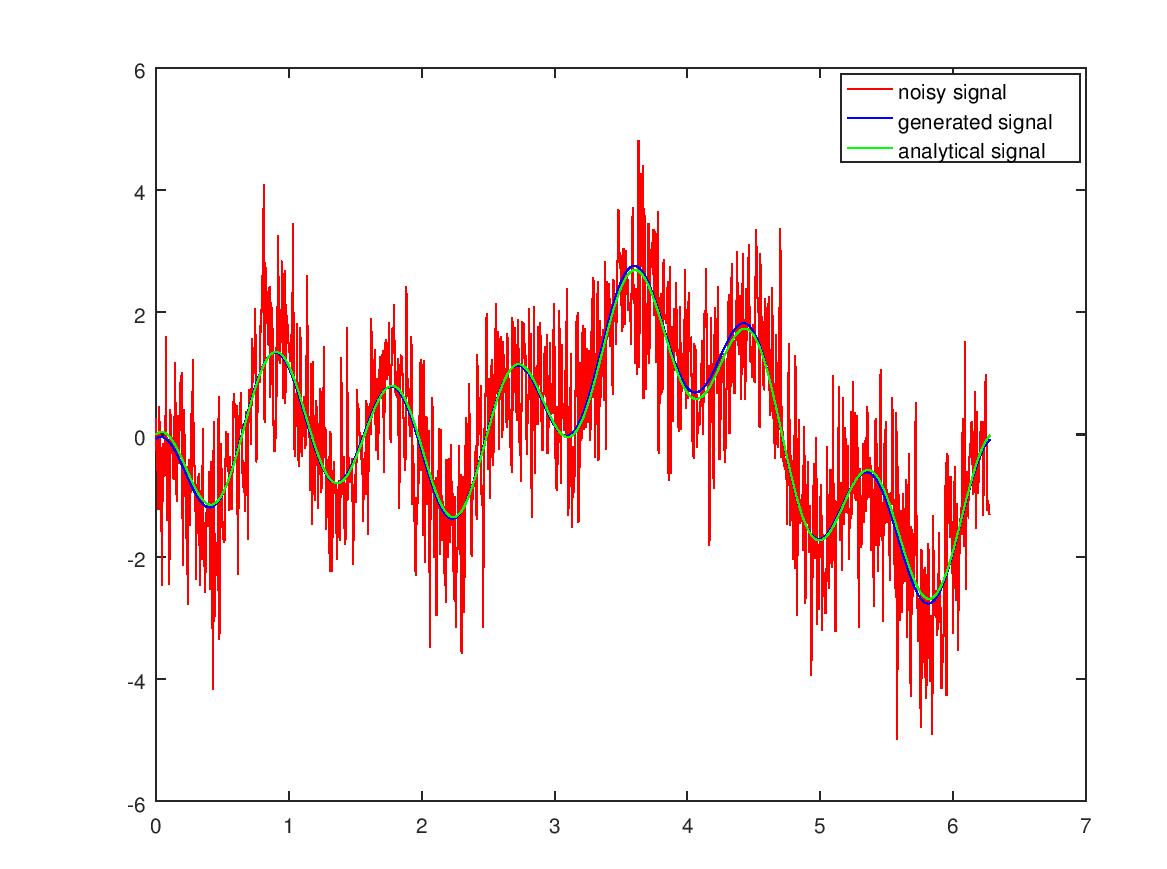
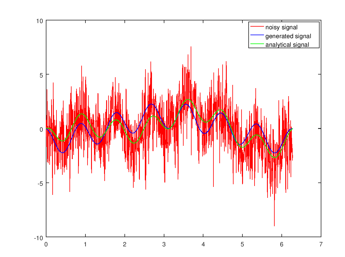
Plot of the generated signal:

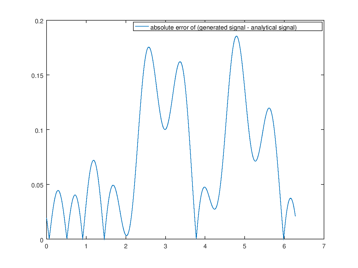
Here is a plot of the absulute error of the generated signal minus the analytical signal.

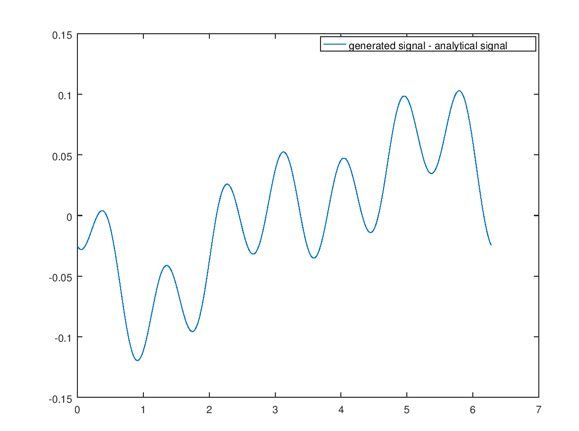
and the relative error (discrepancies between the two result from different added noises)

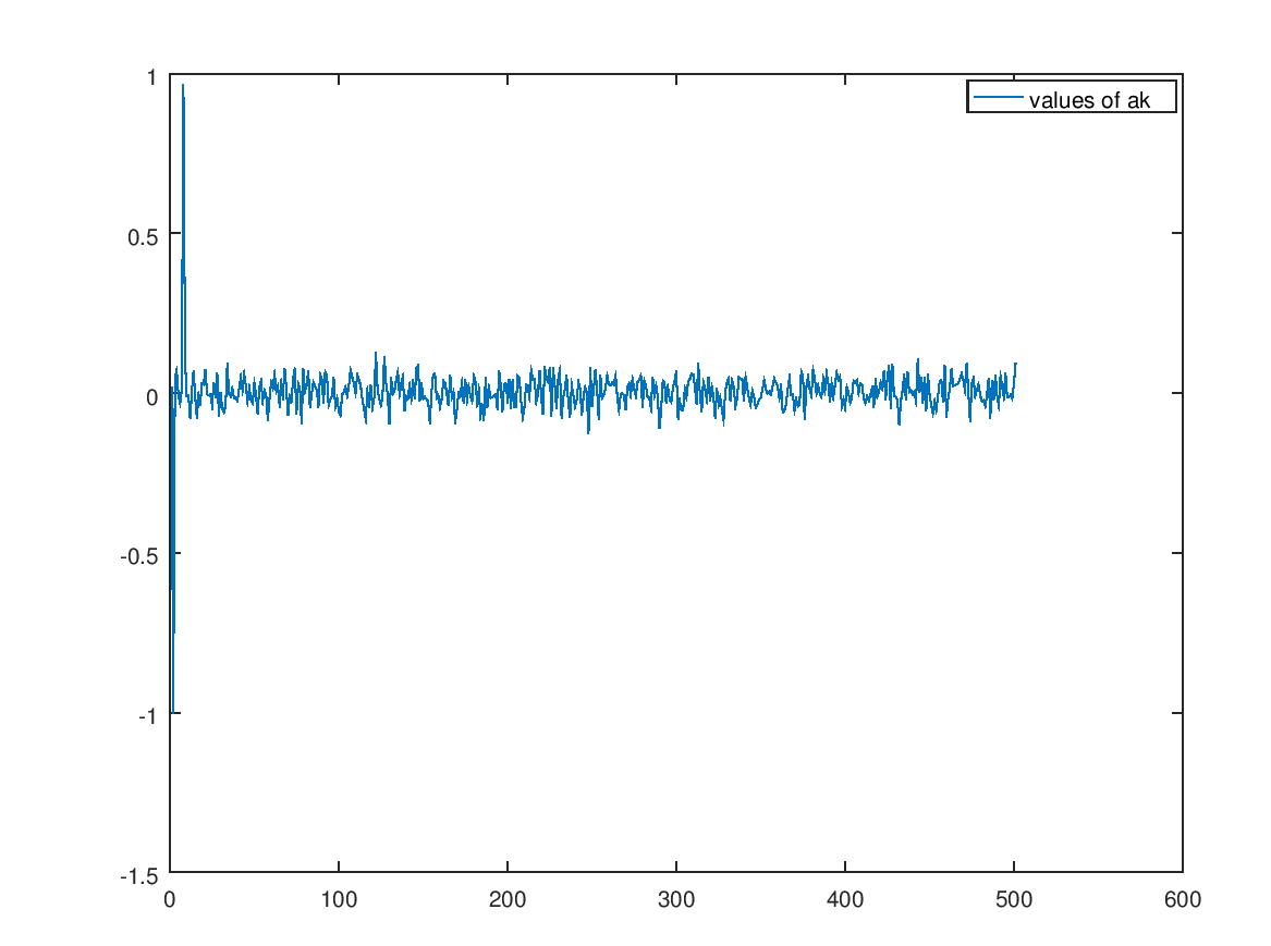
These are the ak values if the ck values weren’t filtered. After the filtering all the values near zero are exactly zero. This removes the noise from the generated signal.

This is what the generated signal looks like without the filtering of the fourier coefficients.

Doubling the noise also results in a subpar result:

Reducing the percantage of fourier coefficients to the top 5% however improves the result again: